Tutorial
IMSEQ comes with three example input files and the reference segment files for the human T cell receptor alpha (TRA) and beta (TRB) chain genes.
- Example 1: Simulated error-free data
- Example 2: Low quality real world data
- Example 3: PCR Barcode Correction
Example 1: Simulated error-free data
The first example is an error-free simulated dataset of 50 full gene sequences. The data can be found in examples/data/example_sim.fa. To process the data, IMSEQ can be invoked as follows:
$ imseq -r -ref ../Homo.Sapiens.TRB.fa -o output.tsv data/example_sim.fa
The -ref option is used to tell IMSEQ where to find the FASTA file with the correctly formatted V and J segment sequences. With -o we instruct IMSEQ to write an output file with detailed information about every successfully processed read. The last argument passed to IMSEQ is the input file.
IMSEQ assumes that the TCR amplicon will have the orientation as shown in the figure above. That means that normally, the V segment is sequenced on the forward strand (for paired end reads) and the V(D)J reads are sequenced on the reverse strand, and single-end reads are always sequenced on the reverse strand. The -r switch reverses this behavior, and is used in this example because the sequences in example_input_sim.fa have been simulated on the forward strand.
The file output.tsv now contains TAB separated information about every input read:
seqId    cdrBegin  cdrEnd  leftMatches  leftErrPos  leftMatchLen  rightMatches  rightErrPos  rightMatchLen  cdrNucSeq                                cdrAASeq
READ-1   273       300     V16          -           276           J2-7          -            31             TGTGCCAGCACCTACGAGCAGTACTTC              CASTYEQYF
READ-10  270       303     V6-2V6-3     -           273           J2-4          -            31             TGTGCCAGCATTTCCAAAGACATTCAGTACTTC        CASISKDIQYF
READ-11  270       297     V3-1         -           273           J2-1          -            31             TGTGCCTGCTACAATGAGCAGTTCTTC              CACYNEQFF
READ-12  273       303     V7-4         -           276           J2-1          -            31             TGTGCCGGCTGCTTAGATGAGCAGTTCTTC           CAGCLDEQFF
READ-13  273       312     V23-1        -           276           J2-6          -            31             TGCGCCAGCAGGCAATCTGAGGCCAACGTCCTGACTTTC  CASRQSEANVLTF
The file format is explained in the ouput files documentation.
Example 2: Low quality real world data
The second example file contained in the IMSIM downloads is examples/data/example_quality_bias.fq.gz. It originates from a low quality sequencing run and illustrates the impact of low quality reads on the clonotype distribution when they are filtered out. We will process the data twice, once with a quality threshold of 30 and no posterior clustering and once with a quality threshold of 10 with posterior clustering:
$ imseq -ref ../Homo.Sapiens.TRB.fa -j 4 -mq 10 -qc -oa MQ10QC data/example_quality_bias.fq.gz
$ imseq -ref ../Homo.Sapiens.TRB.fa -j 4 -mq 30 -oa MQ30 data/example_quality_bias.fq.gz
This time, we do not write a full per-read output file but aminoacid based clonotype counts (-oa). IMSEQ shall also use 4 parallel threads (-j 4). A clonotype count output file look like this:
$ sort -rnk2 MQ30 | head
V20-1:CSARDELAANYEQYF:J2-7       343
V6-5:CASSYSTGVIDGYTF:J1-2        287
V6-5:CASSFQTGTGVYGYTF:J1-2       158
V12-3V12-4:CASSTQGYEQYF:J2-7     65
V10-3:CAVRLAGETDTQYF:J2-3        56
V6-1:CASRGYNEQFF:J2-1J2-5        43
V27:CASSPTSGAPGEQFF:J2-1J2-5     43
V12-3V12-4:CASSAQETQYF:J2-5      42
V2:CASMAGTYNEQFF:J2-1J2-5        38
V12-3V12-4:CASSAQETQFF:J2-1J2-5  35
It contains one row for each clonotype associated with its count, separated by a TAB character. This data can be used to examine the two different clonotype distributions generated with the two different parameter sets. We provide a small R script in the examples directory, examples/top10PlotPDF.R, which visualizes the frequencies of the top 10 clonotypes in a bar diagram. It is invoked as follows:
$ ./top10PlotPDF.R MQ10QC MQ30 MQ.pdf
The output file, MQ.pdf, should contain the following plot:
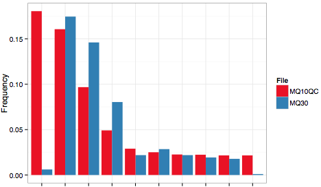
The example clearly shows that a simple quality filtering approach can drastically change the clonotype distribution and indicates that erroneous reads should rather be rescued and corrected than discarded.
Example 3: PCR Barcode Correction
The third example provided with IMSEQ is a real data file from a sample
that was prepared with PCR barcodes. During an initial liniar amplification
step, 10 random nucleotides were inserted along with the reverse primer, hence
the V(D)J read starts with those 10 random nucleotides. At first, we perform a
standard analysis, ignoring the barcode. We specifcy -bcl 10 in order to
indicate that the first 10 bases are barcode and have therefore to be ignored
for the clonotyping analysis, but we also specify -ber 0 in order to
prevent barcode based clustering:
$ imseq -ref ../Homo.Sapiens.TRB.fa -j 4 -oa NO_BC -bcl 10 -ber 0 data/example_barcode_correction.fq.gz
Now, we analyse the same data but enable the barcode based correction. We write two files, one with the read counts per clonotype (-oa) and one with the barcode counts per clonotype (-oab):
$ imseq -ref ../Homo.Sapiens.TRB.fa -j 4 -oa BC -oab BC_NORM -bcl 10 data/example_barcode_correction.fq.gz
Comparing the files NO_BC and BC shows, that the barcode based correction reduced the number of clonotypes:
$ wc -l BC NO_BC
575 BC
615 NO_BC
A comparison of distribution of the top 10 clonotypes can be visualized using the provided R script:
$ ./top10PlotPDF.R NO_BC BC BC_NORM BC.pdf
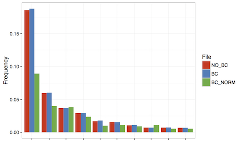
Two observations can be made: Firstly, clustering clonotypes based on the barcode information slightly increases the frequency of the top 10 clonotypes since the erroneous clonotypes in the tail of the repertoire distribution are assigned to their correct original clonotype. Secondly, if one computes the distribution based on the barcode counts rather than based on the read counts, the distribution flattens significantly, indicating that the most dominant clonotypes were boosted through preferential amplification. Rank shifts can already be observed among the top 10 clonotypes.